For this month’s data visualization challenge, I identified some possible analyses to build on my Ohio voter file dataset I build last month.

In this first update, I have conducted exploratory analysis to find further insights in the data.

For example, let’s say you are the Ohio Democratic Party. You want to ensure you mobilize voters that defected from the GOP after the election of Donald Trump. They may ask, “Where do these voters live?”

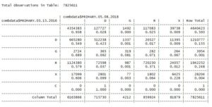
To do this, we can use the Ohio dataset I mentioned above. Let’s look for residents that voted in the 2016 GOP Primary but the 2018 Democratic Primary. How many of them are they?

crosstab_primaries <- CrossTable(combdata$PRIMARY.03.15.2016, combdata$PRIMARY.05.08.2018,
prop.r = TRUE, prop.c = FALSE, prop.chisq = FALSE, prop.t = FALSE)

Using the CrossTable command above, we find that there are 20,527 such voters.

 

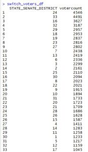
Using some data manipulation and the dplyr package, we can identify the state senate districts these voters are most commonly in.

switch_voters_to_target <- combdata[combdata$PRIMARY.03.15.2016 == “R” & combdata$PRIMARY.05.08.2018 == “D”,]

head(switch_voters_to_target)

switch_voters_senate_districts <- switch_voters_to_target %>%
group_by(STATE_SENATE_DISTRICT) %>%
summarise(votercount = n()) %>%
arrange(desc(votercount))

switch_voters_df <- as.data.frame(switch_voters_senate_districts)

They are primarily in Ohio state senate districts 24, 33, 16, and 32.

If we look at where these districts are, they fit a larger national trend that affected the GOP in 2018.

• District 24 is in the suburbs of Cleveland.
• Districts 32 and 33 contain Youngstown and its suburbs.
• District 16 is in the suburbs of Columbus.

Suburban, white women abandoned the GOP in 2018. This is due to a combination of Trump’s sexual assault allegations, Brett Kavanaugh, and the GOP tax bill capping State and Local Tax (SALT) deductions at $10,000 (which hurts affluent property owners).

I hope to build on this analysis for my final visualization.